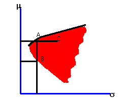
Graphically, our goal is to characterize the set of portfolios that lie on the efficient frontier region, extending northeast from the vertex of the investment opportunity set in Figure 4.3.
|
Figure 4.3 |
|
Investment Opportunity Set |

Recall the statistics associated with the expected return distribution for the Three-Firm Case.
|
Firm |
Expected Return |
Return Variance |
Covariance (i,j) |
(i,j) Pair |
|
Firm 1 |
0.229 |
0.924 |
0.063 |
(1,2) |
|
Firm 2 |
0.138 |
0.862 |
-0.582 |
(1,3) |
|
Firm 3 |
0.052 |
0.528 |
-0.359 |
(2,3) |
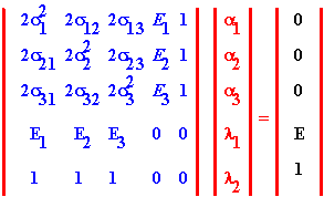
Recall that the matrix representation of the three-firm problem derived in topic 4.8, and provided in table 4.1 is the following:

which is more conveniently denoted as:
V A = W
Substituting the values from the three-firm problem, the V matrix becomes:
|
2(0.924) |
2(0.063) |
2(-0.582) |
0.229 |
1 |
|
2(0.063) |
2(0.862) |
2(-.359) |
0.138 |
1 |
|
2(-0.582) |
2(-0.359) |
2(0.528) |
0.052 |
1 |
|
0.229 |
0.138 |
0.052 |
0 |
0 |
|
1 |
1 |
1 |
0 |
0 |
Let the vector of variables being solved for be denoted as A
|
a 1 |
|
a 2 |
|
a 3 |
|
l 1 |
|
l 2 |
and the product of VA be denoted as W.
|
0 |
|
0 |
|
0 |
|
E |
|
1 |
The inverse of V is given by:
|
0.097 |
-0.198 |
0.101 |
6.228 |
-0.460 |
|
-0.198 |
0.405 |
-0.207 |
-1.153 |
0.338 |
|
0.101 |
-0.207 |
0.105 |
-5.075 |
1.122 |
|
6.228 |
-1.153 |
-5.075 |
-164.523 |
20.339 |
|
-0.460 |
0.338 |
1.122 |
20.339 |
-2.535 |
Pre-multiplying W by V
-1 (see topic 4.8) yields the general expression for minimum-variance portfolio weights as a function E for stocks 1,2, and 3.Firm 1 = 6.288E - 0.460
Firm 2 = -1.153E + 0.338
Firm 3 = -5.075E + 1.122
For example, if the desired expected return is 0.14 (i.e., 14%), then substituting 0.14 for E above yields the minimum-variance portfolio weights.
|
Portfolio |
Weights |
|
Firm 1 |
0.41 |
|
Firm 2 |
0.18 |
|
Firm 3 |
0.41 |
The next part of this chapter lets you read about properties associated with the shape of the frontier.
previous topic
next topic
(C) Copyright 1999, OS Financial Trading System